|
|
|
|
|
Statistics and system tools |
 |
|
|
|
 |
|
Requirements of Statistical
Inference
The basic tenet of statistical inference is to use information gathered on a
portion of the population of interest, a sample, to estimate characteristics of
the population as a whole. In other words, we aim to make generalisations about
the target population we are interested in on
the basis of a smaller, manageable sample. In this special case, we are
interested in estimating distant disease-free and disease-specific survival for breast cancer patients, and we
use for this purpose a data set collected as a nationwide project in Finland. |
|
To make a dependable
generalisation or prediction, the data set must be representative of the target
population. In the present study 91% of all breast cancer cases diagnosed within
the selected regions and the chosen time interval could be included in the
database, which might suggest that the series is relatively unbiased.
Top of page |
|
|
|
Requirements of Survival
Analysis
In the special case of survival analysis, not all persons are observed for the
full time to event, here distant recurrence or death from breast cancer. If a
person dies of an intercurrent reason (other than breast cancer) or is lost to
follow-up before experiencing the event of interest, he or she is said to be
censored from the analysis when last observed. Survival analysis is specifically
designed to summarise time to event data with censoring, and the resulting
estimate will not be biased by being based on shorter follow-up and fewer deaths
-provided that three basic requirements hold true:
|
|
· Correct recording of time of entry into the study
· Correct recording of time to event or loss to follow-up
· The assumption that a patient's chance of being lost or
withdrawn is
unrelated to his risk of distant recurrence or
death from breast cancer.
If any of these conditions is not met, serious bias in the survival curve and
any comparisons based on the data set will result.
Top of page |
|
|
|
Survival curves according
to the Kaplan-Meier product-limit method
The purpose of a life-table is to estimate the percentage of patients who
survive and do not experience an event, such as in this case distant recurrence
or death from breast cancer, within a chosen population and during a given
period of follow-up time. An inherent feature that has to be taken into account
in any survival analysis is that many patients die of causes unrelated to the
specific disease that is being studied, are lost to follow-up, or are still
alive at the end of the study period. In these cases we do not know whether they
will eventually suffer from a recurrence or will die of breast cancer, and they,
therefore, have to be treated by a mathematical method called censoring. This
method makes use of the available information, so that these subjects contribute
information to outcome calculations until the last time point of follow-up.
|
|
The survival curve is drawn as
a step function, since the percentage surviving individuals remains unchanged
between any two events, even if there are censored observations between the
events. At the time zero, by definition, all patients are alive, so the survival
estimate is 100%. Time zero is not some specified calendar date; but it is the
time when each patient entered the study, and in this specific case the time
zero is the time of the diagnosis of the primary breast cancer.
The survival curve has a
downward step whenever an event occurs. The set of times at which the curve
shows a step is simply the set of uncensored event times in the dataset.
Top of page |
|
|
|
How to calculate a
life-table according to Kaplan-Meier
The probability of surviving a given period of time can be calculated by
considering time to consist of many small intervals of similar duration (e.g.
days). For example, the probability of an individual to survive for 30 days can
be considered to be the probability of first surviving for 29 days, multiplied
by the probability of surviving the 30th day (see the example given below). To
calculate the probability, the number of individuals who survived beyond the
30th day is divided by the number of individuals who were alive at the beginning
of the day 30 (this is the number of patients who survived beyond the 30th day +
the number of patients who died during the day 30. In this method those
individuals who died of an intercurrent cause during the day 30 are excluded
(censored)
|
|
on that day from both the numerator and the denominator. Thus, this method
automatically accounts for the censored patients, since both the numerator and
the denominator are reduced on the day when the intercurrent death took place.
Because we calculate the product of many successive survival probabilities (e.g.
the probability to survive each day of follow-up), this method is also called
the product-limit method. The graph (survival curve) corresponding to the
life-table is also shown at the website (see Figure 1).
An example of computation of a
life-table in a series of 51 patients in given below:
|
|
Figure 1. A graph corresponding to the
life-table
|
|
Interpretation of survival
curves often involves mistaken over-interpretation of the right-hand part of the
curve. It is common for a survival curve to flatten out after an initial slope
as events become less frequent. It is unwise to interpret such a plateau as
meaningful unless there are many subjects still at risk. The life-table survival
estimates become increasingly unreliable as the number of patients at risk
decreases (i.e. the number of patients still being followed up becomes less). In
general, it has been recommended that the tails of survival curves should not be
drawn when the number of subjects still at risk falls below five.
Confidence intervals can also
be calculated for the survival |
|
percentages. First, we need to
calculate the standard error. A simple formula for the standard error (SE)
is
where pk is the estimated
percentage surviving at time k and rk is the number of subjects still at
risk at time k. Assuming that pk will have an approximately normal sampling
distribution, we can calculate a 95% confidence interval for pk as pk -
1.96SE(pk) to pk + 1.96SE(pk).
Top of page |
|
|
Comparison of two survival
curves
The
logrank test
Visual comparison of two survival curves is informative, but a more objective
significance test may also be needed to assess the evidence for a true survival
difference between the selected patient groups.The most commonly used test to
compare two survival curves is called the Mantel-Cox logrank test, which
compares the observed number of events with the number expected in the groups,
assuming that there is no survival difference between the two groups of patients
(this is called "the null hypothesis"). In other words, if no survival
difference existed between the groups, then at any interval or point of time,
the total number of events should be divided between the groups in a proportion
to the number of patients at risk. For example, if the chosen |
|
Profile 1 and Profile 2 in the
case-match system have the same number of patients, then each group should
have about the same number of events during any observed time interval. On
the other hand, if the number of patients in Profile 1 is twice as large as
2, then there should be two times more events in Profile 1 if the outcome in
both groups was similar. The comparisons between the groups are calculated
at each event time, and this information is then combined across all event
times.
The logrank
test gives an equal weight to all event times and is best suited to detect
differences between survival curves for which the underlying hazard
functions are proportional. Alternative weighting can be achieved by using
e.g. the Peto test, which gives greater weight to early events.
Top of page |
|
|
|
How to calculate the logrank
test
The main task is to calculate
the number of events expected in each group if we assume that there were no
difference. One first needs to rank the survival times of all events (both
groups combined) in an ascending order (see Table 1). For each event time, t,
one needs to record the number of events at that Profile 1 and Profile 2 in the
case-match system have the time, dt , and the number of patients alive (at risk)
up to that event time in each group, n1 and n2. Therefore, for each event time
there are small contributions e1 and e2 to the expected number of events. The
expected number of events in group 1 at a particular event time is then defined
as:
Then the expected number of
events in group 1, E1, across all event times is the sum of all contributions,
e1, defined as:

|
|
and the corresponding observed
number of events in group 1, O1, is defined as:

Then the logrank test statistic
is defined as:
This chi-square value is
converted to a p-value in the same way as in a conventional chi-square test.
Hence using Table 1 we get

Thus, the logrank test showed a
significant survival difference between the group 1 and the group 2.
|
|
Table 1. Calculation of the number of
expected (e) and observed (o) events in two groups, n1 and n2, ranked according
to the survival times. In group 1, one patient was lost to follow-up at 75
months and was thus censored
|
|
|
Case-match calculation
All personal identification information was deleted and replaced by internal
coding when the database was assembled. The user can enter a prognostic factor
profile of choice by selecting any of the available categories in the drop-down
lists. A query is subsequently automatically performed to the FinProg breast
cancer database to retrieve the data of the patients with a matching prognostic
factor profile and known outcome. The distant disease-free survival (DDFS) or
optionally disease-specific overall survival is calculated according to the
Kaplan-Meier product-limit method on the server using actual survival data of
all matching patients. DDFS is calculated from the date of the diagnosis to the
occurrence of metastases outside the locoregional area. Patients who died of
breast cancer without any record of recurrence (4% of breast cancer deaths) are
analysed as though they had a recurrence at the time of death. Patients who died
of other causes than breast cancer or |
|
were lost to follow-up are censored. Only
exact matching according to the pre-defined prognostic factor categories in the
drop-down lists is performed, and no nearest-neighbour or other corresponding
techniques are applied.
The results are displayed as a survival curve supplemented by a table showing
the corresponding percentages of surviving patients and the numbers of patients
at risk at specified time points (figure 1). Optional results include the
confidence intervals for the Kaplan-Meier estimates and the median survival
time, if obtainable, for the selected prognostic factor profile (table 1). The
distribution of patients according to disease status (alive without recurrence,
with recurrent disease or dead of breast cancer, and dead of intercurrent
causes) within a selected profile and at a certain time-point can also be
displayed as a table or chart of choice. Two factor profiles can be visually and
statistically compared on the website by clicking the "two profiles"
option and the checkbox for the logrank test. |
|
Figure 1. A Kaplan-Meier life-table of
survival. From this graph it is possible to estimate the cumulative survival at
a specific time point, for example five years of follow-up (red arrows) or the
median survival time, corresponding to the time point at which half of the
patients (50% cumulative survival) remain at risk (blue arrows)
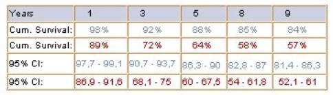
Table 1. Kaplan-Meier results for the two
selected profiles, including standard errors, confidence intervals and the
median survival
Top of page |
|
|
|
References 1.
Altman DG. Practical statistics for medical research. 1st Ed. London: Chapman
& Hall; 1991
2.
Kleinbaum DG. Survival analysis: a self-learning text. New York:
Springer-Verlag; 1996
|
|
3. Pocock SJ. Clinical trials: a
practical approach. John Wiley & Sons; 1983 |